Why are IQ test results normally distributed?
(I'm a nooby in probability)
So why are IQ test results normally distributed? Or more precisely what are the hypothesizes and theorems that imply this distribution?
Has it to do with the central limit theorem? (But this theorem is about the arithmetic mean of iid variables. I dont see iid variables here: I suppose it's not one person repeating the test. Is it the skills given at a person that is considered as a random variable?)
$\endgroup$ 103 Answers
$\begingroup$As Ron Maimon has said in the comments, the IQ scale is defined so that it gives a normal distribution with mean $100$ and standard deviation $15$. This is possible for any test score with a continuous distribution $f$. If the subject's score in the test is $s$, their IQ will be given by:
$$\text{IQ}=100+15\sqrt 2\;\text{erfc}^{-1}\left(2-2\int_{-\infty}^sf(x)dx\right)$$
To see that this gives a normal distribution, invert the equation above:
$$\int_{-\infty}^sf(x)dx = 1 - \frac{1}{2}\;\text{erfc}\left(\frac{\text{IQ} - 100}{15\sqrt 2}\right)$$
The left-hand side is the cumulative distribution function (CDF) of the test scores and the right-hand side is the expression for the CDF of a normal distribution.
It may sound weird to define IQ so that it fits an arbitrary distribution, but that's because IQ is not what most people think it is. It's not a measurement of intelligence, it's just an indication of how someone's intelligence ranks among a group:
The I.Q. is essentially a rank; there are no true "units" of intellectual ability.
[Mussen, Paul Henry (1973). Psychology: An Introduction. Lexington (MA): Heath. p. 363. ISBN 978-0-669-61382-7.]
In the jargon of psychological measurement theory, IQ is an ordinal scale, where we are simply rank-ordering people. (...) It is not even appropriate to claim that the 10-point difference between IQ scores of 110 and 100 is the same as the 10-point difference between IQs of 160 and 150.
[Mackintosh, N. J. (1998). IQ and Human Intelligence. Oxford: Oxford University Press. pp. 30–31. ISBN 978-0-19-852367-3.]
When we come to quantities like IQ or g, as we are presently able to measure them, we shall see later that we have an even lower level of measurement—an ordinal level. This means that the numbers we assign to individuals can only be used to rank them—the number tells us where the individual comes in the rank order and nothing else.
[Bartholomew, David J. (2004). Measuring Intelligence: Facts and Fallacies. Cambridge: Cambridge University Press. p. 50. ISBN 978-0-521-54478-8.]
From those quotes you can deduce that any other information about the original distribution of scores in the actual test used to measure intelligence, like skewness and kurtosis, is simply lost.
The reason for choosing a gaussian, and with those parameters, is mostly historical. But it's also very convenient. It turns out that you'd need about as many people as have ever existed to get someone to be ranked as an IQ of zero and someone else to be ranked as $200$ (roughly $1$ in $76$ billion). So in practice IQ is limited to the interval $[0, 200]$ (no, there's no such thing as $300$ IQ. Sorry Sidis). Also, the dumbest person alive would have an IQ of $5$ and the smartest person $195$ ($1$ in $8.3$ billion). If you could theoretically apply the same test to trillions of people, then you'd get IQs above $200$ and even negative IQs. Obviously the results will be different for different tests, and you might question whether any of the tests have really anything to do with actual intelligence.
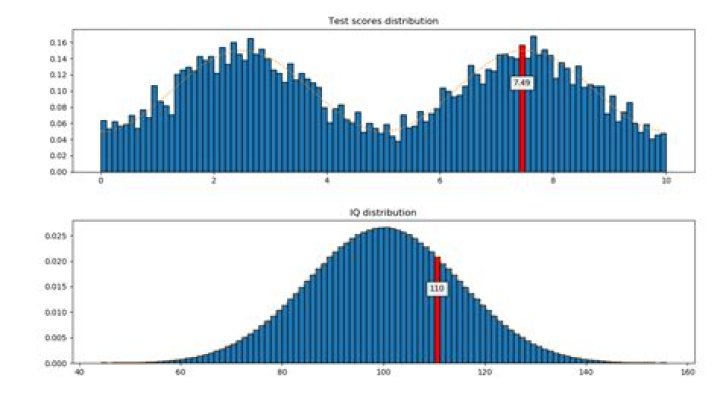
To illustrate how you'd calculate IQ in practice, I made a Python script which takes an arbitrary distribution of scores in a test, generates a sample of $10$ thousand results and uses that to calculate the IQ of an additional participant based on their score in the same test. The plot shows the distribution of scores and how it's transformed into a normal distribution when converted to IQ. The score and IQ of the new participant is shown in red.
import bisect
import numpy as np
from scipy.special import erfcinv
from scipy.stats import rv_continuous
N_SAMPLES = 10000
np.random.seed(0)
# Start with any continuous distribution for the test scores.
# In this case, it's a multimodal distribution.
def scores_pdf(x): return (2-np.cos(2*np.pi*x/5))/20
class dist_gen(rv_continuous): def _pdf(self, x): return scores_pdf(x)
# We restrict the score to be between zero and ten.
dist = dist_gen(a=0, b=10)
scores = dist.rvs(size=N_SAMPLES)
scores = list(sorted(scores))
# Convert from percentile to IQ
def p_to_iq(p): return 100 + 15*np.sqrt(2)*erfcinv(2 - 2*p)
# The scores are not even used yet, only their ordering.
iqs = [p_to_iq(k/N_SAMPLES) for k in range(1, N_SAMPLES)]
# Calculating the percentile for a finite sample set depends on
# how it is defined. This function returns the smallest and the
# highest values.
def get_percentile_bounds(score): size = len(scores) # Number of samples lower than 'score' lower = bisect.bisect_left(scores, score) # Number of samples greater than 'score' greater = size - bisect.bisect_right(scores, score) return lower/(size+1), (size-greater+1)/(size+1)
# We use only the definition of percentile closest to the average.
# (This is arbitrary and irrelevant for large sample sets)
def get_iq(score): p1, p2 = get_percentile_bounds(score) if abs(p1-0.5) < abs(p2-0.5): return p_to_iq(p1) return p_to_iq(p2)
# A new subject performs the test.
new_score = dist.rvs()
new_iq = get_iq(new_score)
print(new_score, new_iq)
import matplotlib.pyplot as plt
from scipy.stats import norm as gaussian
N_BINS = 100
def highlight_patch(value, patches, axis, fmt): left, bottom = patches[0].get_xy() width = patches[0].get_width() n = int((value - left)//width) patches[n].set_fc('r') x = left + (n+0.5)*width y = bottom + 0.7*patches[n].get_height() axis.text(x, y, fmt%(value), horizontalalignment='center', verticalalignment='center', bbox=dict(facecolor='white',alpha=0.9))
fig, axes = plt.subplots(nrows=2, ncols=1)
n, bins, patches = axes[0].hist( scores, bins=100, density=True, edgecolor='black')
highlight_patch(new_score, patches, axes[0], '%.2f')
x = np.linspace(scores[0], scores[-1], num=200)
axes[0].plot(x, [scores_pdf(k) for k in x], ':')
axes[0].set_title('Test scores distribution')
n, bins, patches = axes[1].hist( iqs, bins=100, density=True, edgecolor='black')
highlight_patch(new_iq, patches, axes[1], '%.0f')
x = np.linspace(iqs[0], iqs[-1], num=200)
axes[1].plot(x, [gaussian.pdf(k, 100, 15) for k in x], ':')
axes[1].set_title('IQ distribution')
fig.tight_layout()
plt.show()It has been an empirically observed fact that many "naturally" observed traits, like height or IQ, are NOT empirically normally distributed. At the very least they can't be truly normally distributed because they are always non-negative. But even more than that, before non-negativity is violated, it has been observed that the "tails" (values enough standard deviations away from the mean) tend to have higher probability than predicted by a normal distribution for the population, at least for certain traits. The only thing you can say is that if you take many samples and compute the mean, then the empirical mean for the sample should be approximately normally distributed under mild assumptions if you have enough samples (this is the central limit theorem).
As an aside, if you'd like a speculative theory for why many traits appear "somewhat normal", just consider the possibility that many factors affect the trait, e.g. many genetic factors and many environmental factors. If you have many factors and their effects are additive and you don't have too crazy distributions for each factor's effect, and the factors are independent enough, then the accumulated effect should be somewhat normal basically by the central limit theorem.
$\endgroup$ 7 $\begingroup$I suggest the distribution of IQ's may be log-linear (not log-normal). Such distributions often called a Gibbs distribution (who first applied it to the distribution of energy and built a strong foundation for thermodynamics (1878), eg Boltzmann) can be applied to like positive-definite variables that have an 'energy' connotation.
t works for me with natural remotely sensed imagery (hurricanes, sea ice, rough ocean surface, cold front occurrences), even heart beat variation BUT only above some threshold. On occasion the down (below average) side can be also log-normal (not necessarily of the same slope).
I'm looking for some data with a sample size large enough to resolve the large deviations from most probable. If anyone has a good suggestion in that regard, please pass it along.
If it turned out to be the case, and IQ's had a log-linear distribution, I would suggest that the IQ variable is acting as an 'energy'. If so I would ascribe the 'energy' to a person's ability to concentrate/focus (as in the colloquial phrase 'brain energy' which would involve the reduction in confusion/entropy associated with tasks.
$\endgroup$