Plot functions from $\mathbb R^2$ to $\mathbb R^2$

$\begingroup$

Suppose there is a function $f:\mathbb R^2 \to \mathbb R^2$ such that $f(x,y)=(x',y')$.

(For example: $f(x,y)=(x+y,y+2)$).

Can we draw a graph of this function in Cartesian coordinates? Thank you.

$\endgroup$ 4

3 Answers

$\begingroup$

The domain and range of this function constitute four dimensions. Typically, you would plot a subset of the domain and its image on two separate 2D graphs. This is also how you would study the domain and range of complex functions.

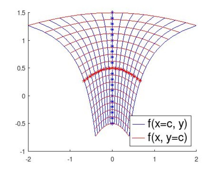
$\endgroup$ 1 $\begingroup$

To elaborate more on D.B.'s answer, you can draw the image of various straight lines (for example) to get some sense on what your map is happening. Here I drew the image of a few lines of the form $x=c$ (blue) and $y=c$ (red) in the square $[-1,1]\times[-1,1]$. I hope you see the effect:

The lines with asterisks are the images of $x=0$ and $y=0$. Here we see that the whole square moved upwards by 2 units and underwent a shear transformation with its upper half stretching linearly to the right (and its bottom -- to the left).

For more complex mappings these straight lines may not give a very descriptive view of what's going on. Anyway, if you want to experiment, here's the octave code I used to generate this picture:

# The transformation to plot
x_hat = @(x, y) x + y;
y_hat = @(x, y) y + 2;
x_breaks = y_breaks = -1 : 0.125 : 1;
# At which points each horizontal (vertical) line will be mapped and drawn.
# A discretized parameter of the curves.
horizontal_lines = -1 : 0.1 : 1;
vertical_lines = -1 : 0.1 : 1;
figure 1; clf; hold on;
# Image of vertical lines at fixed longtitudes
for c = x_breaks xx = arrayfun(@(y) x_hat(c, y), vertical_lines); yy = arrayfun(@(y) y_hat(c, y), vertical_lines); v = plot(xx, yy, ifelse(c, 'b', '-*b'));
end
# Image of horizontal lines at fixed latitudes
for c = y_breaks xx = arrayfun(@(x) x_hat(x, c), horizontal_lines); yy = arrayfun(@(x) y_hat(x, c), horizontal_lines); h = plot(xx, yy, ifelse(c, 'r', '-*r'));
end
legend([v, h], "f(x=c, y)","f(x, y=c)", "location", "southoutside")

You'd get a better feeling probably if you try some more curvy maps on your own, for exmpale with the above code for the map $(x,y)\mapsto(\frac{x}{3 - y},y + 0.5\cos(x))$ I get the following picture:

$\endgroup$ $\begingroup$

Assuming your function f : R²→R² is sufficiently continuous, you can visualize it like this: Let S be an at least 2 dimensional vector space of colors (and/or textures). Let V: R²→S be continuous and (at least locally) 1-to-1. Then V should be a sufficiently nice assignment of colors/textures to the plane to make the color/texture assignment (x,y) →V(f(x,y)) a good visualization of f.

$\endgroup$

Your Answer

Sign up or log in

Sign up using Google Sign up using Facebook Sign up using Email and Password Submit

Post as a guest

Post Your Answer Discard

By clicking “Post Your Answer”, you agree to our terms of service, privacy policy and cookie policy