Linear system control via augmented state space
Consider the simple linear system:$$ \dot{x} = Ax + Bu $$We want to identify a $u$ that ensures x converges to a desired value (typically $0$). Usually this is done by choosing some $u = u(x) = Kx$ so that we end up with $\dot{x} = (A-BK)x$, allowing us choose $K$ appropriately. But, we can instead couple $u$ to the dynamics like this:$$ \begin{bmatrix} \dot{x} \\ \dot{u} \end{bmatrix} = \begin{bmatrix} A & B \\ C & D \end{bmatrix} \begin{bmatrix} x \\ u \end{bmatrix} $$Now we can (theoretically) choose $C$ and $D$ to control the eigenvalues. We'd also need to choose a $u(t=0)$, possibly just setting this to $0$. Note that in order for $x=0$ to be a stable fixed point we need $\dot{x} = Bu = 0$, so we'd likely need $u$ to converge to zero as well.
Intuitively, $u$ acts as an integrator for $x$ with gain $C$, and sometimes LTI systems are given these integrating states to help push $x$ to zero when there are disturbances (not included here). From this point of view, the main difference is that the integrating state $u$ can be made to decay as well by setting $D$.
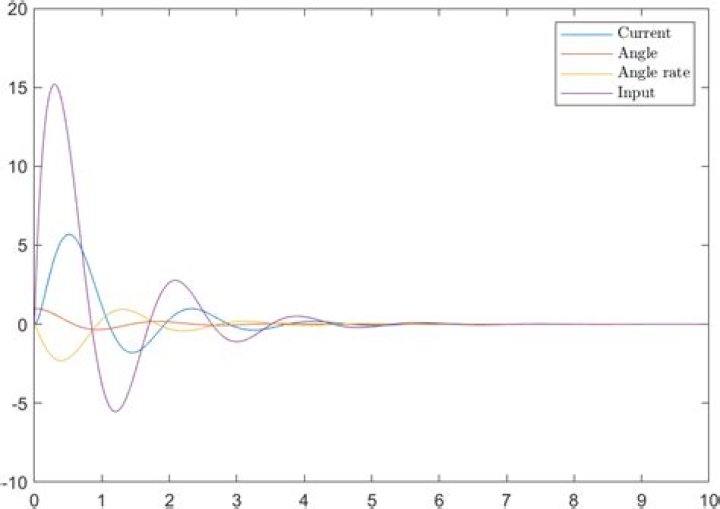
I setup a little experiment with a simple motor model and played around with the values until I got a system where the angle of the motor converged to $0$ (code is below). It seemed to work fine, although it was a bit oscillatory. Here's a plot of that.
I could see this type of model being useful for describing inertia in the input signal $u$.
My questions are as follows:
- Has this already been studied? If so, what is it called?
- When is the system controllable?
- How would you go about designing $C$ and $D$?
I haven't been able to find similar questions or articles on this topic, but please let me know if there's something that I missed!
R= 2.0; % Ohms
L= 0.5; % Henrys
Km = .015; % torque constant
Kb = .015; % emf constant
Kf = 0.2; % Nms
J= 0.02; % kg.m^2
A = [ -R/L -Kb/L 0 % Current 0 0 1 % Angle Km/J -Kf/J 0 % Angular rate
];
B = [ 1/L 0 0
];
C = [0 140 -30];
D = [-10];
A_ = [ A, B ; C, D
];
f = @(t,z) A_*z;
eigvals = eig(A_)
[t,y] = ode45(f,[0,10], [0;1;0;0]);
clf
plot(t,y)
legend('Current','Angle','Angle rate','Input', 'interpreter', 'latex')2 Answers
$\begingroup$Your proposed model alteration is essentially adding an integral before the input
$$ \begin{bmatrix} \dot{x} \\ \dot{u} \end{bmatrix} = \underbrace{ \begin{bmatrix} A & B \\ 0 & 0 \end{bmatrix}}_{\mathcal{A}} \begin{bmatrix} x \\ u \end{bmatrix} + \underbrace{ \begin{bmatrix} 0 \\ I \end{bmatrix}}_{\mathcal{B}} v. $$
In your case you picked $v = C\,x + D\,u$. This is controllable as long as $(\mathcal{A},\mathcal{B})$ is controllable and the matrices $C$, $D$ form a state feedback gain (i.e. choose $\mathcal{K} = \begin{bmatrix}C & D\end{bmatrix}$ such that $\mathcal{A + K\,B}$ is Hurwitz) and one can use different tools to obtain one, such as pole placement or LQR.
$\endgroup$ $\begingroup$It looks a lot like the equation for a double dampener, where the force acting ($F\propto \ddot{x})$ is proportional to the velocity $(\ddot{x}\propto\dot{x}$) but for two dampeners connected with a mass at one end and another end variable, for example.
$\endgroup$