Index Match function in Excel with multiple horizontal criteria

Hope someone can help me with the following Excel task:

Somehow I cannot make it work:

Formula:

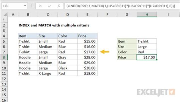
=INDEX($C$2:$C$16,MATCH(F$1,$B$2:$B$16,0),MATCH($E2,$A$2:$A$16,0))

I guess it has something to do with an array formula as it only works one-directional. Can somebody help me out?

1 Answer

Just going off your sample data,

you could just use a SUMIFS rather than INDEX & MATCH

Enter the below into F2, then drag across and down:

=SUMIFS($C:$C,$A:$A,$E2,$B:$B,F$1)

INDEX works by going down then across, using MATCH tells it how far down and across to go.

I.e

• =INDEX(A1:E5,1,1) would give you the value in A1,
• =INDEX(A1:E5,5,1) would give you the value in A5,
• =INDEX(A1:E5,5,5) would give you the value in E5,

Your Answer

Sign up or log in

Sign up using Google Sign up using Facebook Sign up using Email and Password Submit

Post as a guest

Post Your Answer Discard

By clicking “Post Your Answer”, you agree to our terms of service, privacy policy and cookie policy