In a pivot table, how to apply conditional formatting by label instead of by group
In a pivot table you can apply a conditional formatting to a group of value rather than to a cell or to the whole field thank to the "Applies to" option of the "Edit rule" window. My objective here is to make the fill colour change at thresholds that are different for each item rows.
What I would like to do is to reduce the scope of the conditional formatting one more time, to drill down to the label itself.
In the mock-up pivot table below, I would like to apply C.F. to all Class foo rows rather than to the Class field. If the test is Cell value greater than 1, only [Type 1].[Class Foo]|[Category A] and [Type 2].[Class Foo]|[Category B] should change format.
| Pivot talbe Quotas | Column labels | _________________ |
|---|
| Row labels | Category A | Category B |
|---|---|---|
| Type 1 | 13 | 11 |
| __Class Foo | 3 | 1 |
| __Class Bar | 4 | 4 |
| __Class FooBar | 3 | 3 |
| __Class BarFoo | 3 | 3 |
| Type 2 | 8 | 11 |
| __Class Foo | 1 | 5 |
| __Class Bar | 6 | 5 |
| __Class FooBar | 1 | 1 |
For now, I make this work with an AND() function and mixed references but I would like to use icon sets in the future.
The solution can use Power tools but not VBA. Any idea is welcomed, thank you.
1 Answer
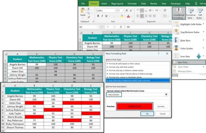
You select the item you want to apply the formatting to, then create the rule.
With your pivot table, if you hover over the left-edge of a row header, you'll see a black arrow. By left-clicking you can select just that class.
Once the class is selected, you create the rule as normal. First:
Then:
As you can see, if you move the classes around, the formatting remains attached to the class.