How to get difference between two dates in random colums in Excel
I have a spreadsheet with about 8000 rows where I have a rowID and 11 columns populated with dates.
Each row has two dates and only two dates;
i.e., the other nine columns are blank.
I want to calculate the difference between the two dates.
It seems awfully inelegant to use a bunch of nested IF functions
to identify the two columns that are not blank.
Is there a straightforward way of doing this?
Any suggestions gratefully accepted.
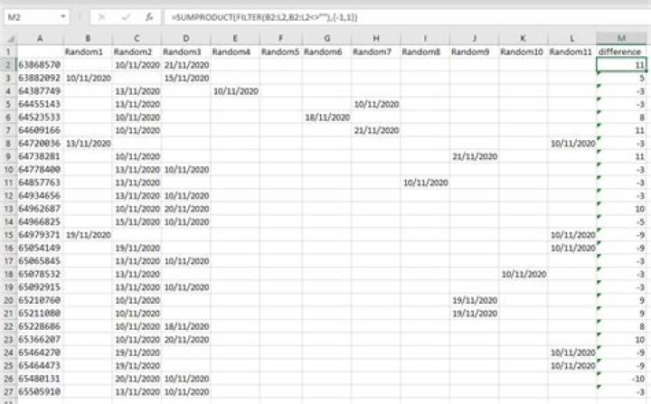
| RowID | Random1 | Random2 | Random3 | Random4 | Random5 | Random6 | Random7 | Random8 | Random9 | Random10 | Random11 |
|----------|------------|------------|------------|------------|---------|------------|------------|------------|------------|------------|------------|
| 63868570 | | 10/11/2020 | 21/11/2020 | | | | | | | | |
| 63882092 | 10/11/2020 | | 15/11/2020 | | | | | | | | |
| 64387749 | | 13/11/2020 | | 10/11/2020 | | | | | | | |
| 64455143 | | 13/11/2020 | | | | | 10/11/2020 | | | | |
| 64523533 | | 10/11/2020 | | | | 18/11/2020 | | | | | |
| 64609166 | | 10/11/2020 | | | | | 21/11/2020 | | | | |
| 64720036 | 13/11/2020 | | | | | | | | | | 10/11/2020 |
| 64738281 | | 10/11/2020 | | | | | | | 21/11/2020 | | |
| 64778400 | | 13/11/2020 | 10/11/2020 | | | | | | | | |
| 64857763 | | 13/11/2020 | | | | | | 10/11/2020 | | | |
| 64934656 | | 13/11/2020 | 10/11/2020 | | | | | | | | |
| 64962687 | | 10/11/2020 | 20/11/2020 | | | | | | | | |
| 64966825 | | 15/11/2020 | 10/11/2020 | | | | | | | | |
| 64979371 | 19/11/2020 | | | | | | | | | | 10/11/2020 |
| 65054149 | | 19/11/2020 | | | | | | | | | 10/11/2020 |
| 65065845 | | 13/11/2020 | 10/11/2020 | | | | | | | | |
| 65078532 | | 13/11/2020 | | | | | | | | 10/11/2020 | |
| 65092915 | | 13/11/2020 | 10/11/2020 | | | | | | | | |
| 65210760 | | 10/11/2020 | | | | | | | 19/11/2020 | | |
| 65211080 | | 10/11/2020 | | | | | | | 19/11/2020 | | |
| 65228686 | | 10/11/2020 | 18/11/2020 | | | | | | | | |
| 65366207 | | 10/11/2020 | 20/11/2020 | | | | | | | | |
| 65464270 | | 19/11/2020 | | | | | | | | | 10/11/2020 |
| 65464473 | | 19/11/2020 | | | | | | | | | 10/11/2020 |
| 65480131 | | 20/11/2020 | 10/11/2020 | | | | | | | | |
| 65505910 | | 13/11/2020 | 10/11/2020 | | | | | | | | |
The dates are displayed above in dd/mm/yyyy format; assume that they are stored as proper Excel dates.
13 Answers
There could be multiple approaches here:
=MAX(B2:L2)-MIN(B2:L2)
- This is probably the simplest formula, this works correctly if you always want to have positive results.
- In case you sometimes need to show negative difference too, then this won't work.
=SUMPRODUCT(FILTER(B2:L2,B2:L2<>""),{-1,1})
FILTERis a very powerful function, introduced recently and available in Office 365.- With this formula you can also respect the order of dates and return negative difference if necessary.
Do
=LARGE(B2:L2,1)-LARGE(B2:L2,2)LARGE will find the largest and second-largest values in the row.
Based on your description of your worksheet,
they will be the two non-blank values.
Use the DATEDIF function if you want (if you have it).
This finds DAYS between two dates form Random Columns in Row:
Formula in cell L2:
=DAYS(SMALL(B2:K2,2),SMALL(B2:K2,1))The DAYS function returns number of days between two dates, here SMALL finds the second & first lowest.
Adjust cell references in the formula as needed.