How to combine a range and cell into a new range within a formula in Excel
I have a formula in Excel that takes an array/range of values as one of the input.
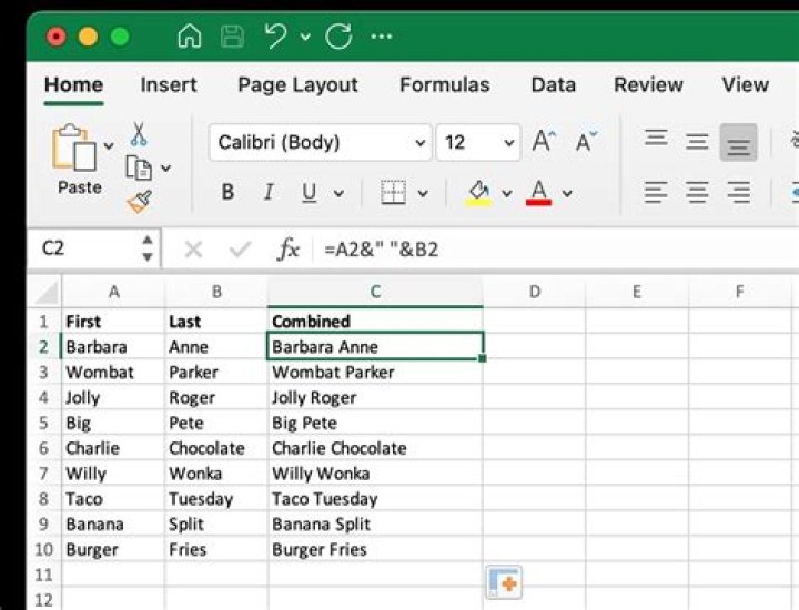
I have a range of values, let's say A1:A6, and a single cell C11. I want to combine the range with the single cell in that exact order, i.e. the result of the combination is an array/range of values will start from A1 to A6 and will end with C11. I don't want the text value by concatenating A1:A6 with C11, rather, I want the array of data containing those in A1:A6 and C11.
For example, in the pic above, I want to apply the array containing the values of A1:A6 and C11 to the formula/function called IRR which takes an array as the first argument.
How can I do that in as part of a formula?
97 Answers
For what it's worth, you can easily accomplish what you're trying to do in Google Sheets using curly brackets: {range1 ; range2} (combining vertically) or {range1, range2} (combining horizontally). This will create a new array of the values from range1 followed by the values from range2 (either vertically or horizontally, depending on whether you separated with a semi-colon or a comma).
For Microsoft Office 2016 only
TEXTJOIN(delimiter, ignore_empty, text1, [text2], …)
In your example, this will be
=TEXTJOIN(" ", TRUE, A1:A6, C11)
The result will be separated by space and it will ignore cells that contain blank value.
Alternate solution
- Select the cell you want the result to be.
- Go to formula bar and enter
=TRANSPOSE("A1:A5")&" " - Select the entire formula and press F9 to convert formula into values.
- Remove curly brackets from both ends.
- Add
=CONCATENATE( result ) - Enter.
If you want to combine a range of values and single cell through the formula you can use $-sign to fix single cell address. For example, when the formula =A1+$C$11 is stretched to the whole range, then in each cell of the range there will be the following =AN+$C$11, where N is the cell number.
The aim is to get Excel to treat the discontinuous range [A1:A6,C11] as one continuous range of 7 cells.
The CHOOSE function can be used. Its syntax is CHOOSE(index_num, value1, [value2], ...). If index_num is 1, CHOOSE returns value1; if it is 2, CHOOSE returns value2; and so on. Also, if index_num is an array, then every value is evaluated when CHOOSE is evaluated.
For this problem, define index_num as an array of 7 numbers, and define the 7 values as cells A1 to A6 plus C11, by writing “=Choose({1;2;3;4;5;6;7},(A1,A2,A3,A4,A5,A6,C11))”. This creates an array of 7 cells one below the other, which take the values from A1 to A6 respectively, with the 7th cell being C11. To get the IRR, just write =IRR(Choose function as described)).
Note that in the Choose function, the numbers 1 to 7 should be separated by semi-colons so as to get a column of 7 numbers; using comma will create a row of 7 numbers. This index_num list may be written as SEQUENCE(7) for those having Office 365. Note that the cell references A1 to A6 and C11 need to be individually specified. Writing A1:A6,C11 does not work.
Vijay L's answer is the way to go. However, you must remove the parentheses around the set of cells CHOOSE() is to act upon:
=Choose({1;2;3;4;5;6;7}, A1,A2,A3,A4,A5,A6,C11 )The reason is that with the parentheses, you have a single thing for CHOOSE() to act upon and since you are telling it to make seven choices, it will return the #VALUE! error for all of them. It won't even do the first one. With this edit Vijay L's method works.
Long strings of cells or ranges like that are obnoxious to type and prone to typos and other errors. You can use a simple technique for building this string of cells:
- Pick a cell that is out of the range
- Press "=" to open the formula editor
- Click on each cell in the order you want it in the listing, typing a comma after each mouse click. Notice a string similar to =A1,A2,A3,A4 develops.
- Verify the chosen cells and if they're correct, highlight the string with your mouse
- Copy it to the Clipboard
- Type in your CHOOSE() function pasting the string within the parentheses, eg. `=CHOOSE(A1,A2,A3,A4)'
If you use this technique in a situation in which immediately pasting it into the function, like here, isn't in the cards, just paste it into a cell near to the formula's cell so it is handy when needed.
An alternative is to use TEXTJOIN() to get a string, then FILTERXML() to burst it back into an array of cells.
=FILTERXML("<Group><Element>"&TEXTJOIN("</Element><Element>",TRUE,A1:A3,C12:C16,TRANSPOSE(C1:D5))&"</Element></Group>","/*/*")This will not work for Excel 2013 due to TEXTJOIN(), and CONCAT(), which can stand in for it, using LEFT(), or another approach, to cut off the "tail" adding a delimiter to it gives its end, started, it's said, in 2017-ish, so maybe not workable in Excel 2016. Those tags are present, so I mention this. Lots of other answers.
If you have a version post-CONCAT, or especially post-TEXTJOIN, making a single column out of disparate one- or two-dimensional ranges, can be done fairly easily, as above.
The formula shows the basic set of issues that arise. There are oddities that require tweaking, but the point here is to give a modern solution for anyone searching.
TEXTJOIN will go across rows, then down, etc. so to achieve the "logical" arrangement for a single column, transpose any 2-D ranges so their columns lie across rows and will remain intact. For simple needs, TRANSPOSE() solves that. For more complex ones, mainly reversing entries for whatever reason, use INDEX() which can handle all four ways one might think of transposing a range, not just the simple one that TRANSPOSE() offers, but for simple needs, use the simple tool!
Once joined, and noting the delimiters were the HTML tags needed between values for FILTERXML() to work, you finish out the string for it by prepending and appending the needed HTML tags to have a single piece of HTML. Then FILTERXML() turns the single array constant into a true array of distinct elements.
Going the more complex direction, bear in mind that FILTERXML() can easily handle multi-HTML-tag-grouped data. So creating the string with, say, and tag sets, which is easily done, would allow you to form the material into two columns or rows (the function defaults to dropping down a column, but TRANSPOSE() pushes it rightward into a row. As many rows as one desires. Just use more pairs. It's far more capable than the usual description of its talents would make it seem.
As for CONCAT(), the use:
=CONCAT(A1:A3)&"K"gives you a concatenation using "K" as a delimiter AND a "K" at the end. You just need to remove the ending "K", what I call a "tail", and you have the same thing. More complicated as you can't "just" specify the ranges and then the "K" just once like with: `=CONCAT(A1:A3,B1:B3)&"K" or you get (say A1:A3 is {1,2,3} and B1:B3 is {"a","b","c"}) "123KabcK" which is no use. Instead:
=CONCAT(A1:A3&"K",B1:B3&"K")specifying the range (which you have to do anyway), then the delimiter, then another range, and so on. In this manner, and in most situations in which you want several sets for FILTERXML() to work on, you actually have more control over the placement of and nature of delimiters in your stringbuilding and might even prefer it to TEXTJOIN().
Finally, FILTERXML() will let you address members of its output array by number: [1], [23776], and so on. Perhaps of more interest, and occasional use, is that [last] is also valid. Add one more way to find, and this time for absolute dead certain, the last item in a column or row. Just place the simple range into the above, and output it (still the same as it was, no changes to it), and address the last cell. So, once in a while, of use that way.
But for the very simple need in the question, CHOOSE() is also dead simple to do. Dead simple is a good thing as there has to be more to life than office work so anything timesaving...
Looking back at a comment, this would also be useful for rearranging an existing column or row, if one had to have a single cell, or several certain cells come first or in various positions, and sorting would not do the trick, nor could one just move them as material to their right, say, would have to move with them and maybe cannot. It would still let you order them virtually, in-formula, the way the SORT() command lets you achieve that without moving anything either. Just break the single range into the single cells and range-like chunks necessary and enter them into your stringbuilder in the appropriate order. For instance, if you have A1:A9 and need A4's data to come first, instead of using the simple string A1:A9, use several elements: A4,A1:A3,A5:A9. The formula doesn't care, so long as you stay in your constructor's limits for parameters. And that can be fudged if really needed.
The set-ups involving CHOOSE as given previously are perfectly good, though have two drawbacks:
- They do not allow a contiguous range to be entered, e.g.
A1:A6 - As such, each individual cell must be referenced as a separate argument within
CHOOSE; for large ranges this could be become a significant inconvenience
An alternative, which does not suffer those drawbacks:
Office 365:
IFERROR(INDEX(A1:A6,SEQUENCE(ROWS(A1:A6)+1)),C11)
All versions of Excel (may require CTRL+SHIFT+ENTER):
IFERROR(INDEX(A1:A6,N(IF(1,ROW(INDEX(A:A,1):INDEX(A:A,ROWS(A1:A6)+1))))),C11)
Note that, in the second formula, the choice of A:A passed to INDEX is arbritrary and has nothing to do with the location of the data. In fact, it could equally be replaced with a reference to any entire column within the worksheet, e.g. B:B, C:C, etc. This construction, being volatile only at workbook open, is preferable to 'fully' volatile alternatives involving INDIRECT or OFFSET.