Excel Mac - create graphs with two columns with values for x- and y-axis

In my Excel-file, I have four columns with information that I want to graph:Sample data

I want to graph this information as follows: the values of t, time, should be the x-axis and the values for A, B and C are the corresponding y-values. I have Excel for Mac, but I can't get this to work. I already searched a lot on the internet, but to no avail. I also need a way to plot e.g. two columns, say that the column with B represents the x-values and the column with A the y-values.

All the points should be connected with each other, like done on the below image.

So how do I create graphs, where I have two (or more) columns for the x- and the y-axis?

Thanks a lot in advance!

2 Answers

the values of t, time, should be the x-axis and the values for A, B and C are the corresponding y-values

The Scatter with Lines could meet your needs. Select the data of Time and columns with A, B and C > Insert Scatter, such as the Scatter with Straight Lines.

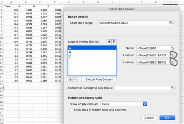
When you need to change the data range for X-axis values and Y-axis values, please right click the chart > Select Data > Select the series that you need to modify, then choose

2

For your first problem (to plot multiple 'y' values), do the following:

• Select all the data that you've arranged like this:

• After that, go to Insert>Scatter and choose a graph type:

• You will have the result on your screen. See this:

For your second problem (to plot 'B' as X and 'A' as Y):

• Without selecting any data, go to insert>scatter and choose a graph type. This will bring a blank graph canvas on your screen.

• Right click on the blank canvas and choose Select Data:

• On the next screen that appears, click Add.

• On the "Edit Series" menu that pops up, enter a series name. I have entered A-B here.

• In Series X values, put =Sheet1!$C$2:$C$11 where $C$2 is the first numeric cell of the data column B (which you want as X axis) and $C$11 last in my case. You have to adjust these values in your case. For example, if C20 is your last numeric cell in data column B and C2 first, change the given formula to: =Sheet1!$C$2:$C$20 where Sheet1 refers to the sheet name.

• Similarly, put in the values of Series Y, as shown below:

• Press 'OK' and then again 'OK' on the menu that appear. That's it. You'll have your desired graph right there.

I hope this helps. Do tell how it does :)

3

Your Answer

Sign up or log in

Sign up using Google Sign up using Facebook Sign up using Email and Password Submit

Post as a guest

Post Your Answer Discard

By clicking “Post Your Answer”, you agree to our terms of service, privacy policy and cookie policy