Excel: First Column Banded in an table

Banded rows and Banded columns in excel is very helpful. But I want to create a table in which I want Banded Column in which only the first column is banded.

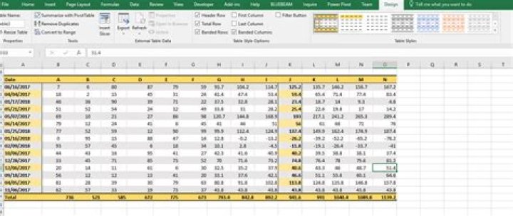
I've tried using the Banded Columns and increasing the steps in second column stripe, but excel only allows a maximum of 9 steps(Screenshot below)

I tried using the first column button, but it doesn't give me banded rows

1

1 Answer

Edit based on OP comment:If you want banded rows to be a different color in just the first column, you can use conditional formatting.

Select the cells you want to have unique banding, click on "Conditional Formatting" > New Rule > Use a Formula To Determine Which Cells to Format.

Enter this in the formula:

=MOD(ROW(),2)=1

Click "Format" and choose a fill color of your choice. I went with yellow again and got the following:

You may just need to extend the formatting if you add new rows.

Original AnswerKeeping the following in the event someone needs info on First Column Banding. If you only want the first column to be colored, you don't want "banded columns" you want "First Column". It's a check box above the Banded Columns box you have selected in your screenshot.

You can either right click on the table theme you have selected in the "Table Styles" section of the ribbon and hit "Modify" (begin at step 3 below), or follow all these steps to create a new style:

Step 1 - click on the down arrow with the horizontal line over it in the Table Styles section.

Step 2 - Then select "New Style"

Step 3 - Then, select "First Column" and format it with the color of your choice. Here I made it yellow so it stood out in the picture.

Now your new style will be in the Table Styles section in the Ribbon. Just make sure you have "First Column" selected.

Second Edit based on OP Comment

If you do not want to use conditional formatting, the only other way I know of would be to use a "helper table"

In the example below, I added a table in Col A with A2 having the formula =B2

Then I dragged that table down to match the length of the data table, and the formula prefills. Next, I hid the date field from the data table, and formatted the colors of each table uniquely. You could change the header bar color using the formatting steps in my original answer above.

You may need to play with the formula to account for rows in the data table not showing if someone filters the data, but the dates should continue to match if the data table is sorted.

Hope this helps!

4

Your Answer

Sign up or log in

Sign up using Google Sign up using Facebook Sign up using Email and Password Submit

Post as a guest

Post Your Answer Discard

By clicking “Post Your Answer”, you agree to our terms of service, privacy policy and cookie policy