Excel colon in function
I am learning excel functions and modeling from Google and trial and errors so just want to clarify the following point to get my fundamental understanding correct:
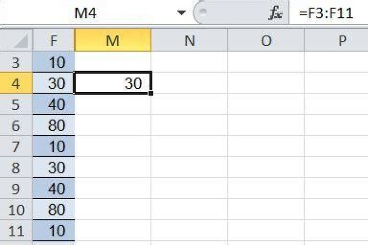
When it comes to colon in excel, I understand that it means defining a range of cells, but when I enter =F3:F11 excel gives the result 30. May I know why is that so? I was trying to interpret it using average / mode etc. and evaluated the formula but fail to find any logical meaning behind it.
2 Answers
F3:F11 is a range, but you're entering it in a place where it's only appropriate to give a single value, so Excel tries to choose one value from the range, using the following rules:
- If the range is in a single column (as this is) Excel chooses the cell from that column in the same row as the referring cell (or the error
#VALUE!if the range doesn't intersect that row) - If the range is in a single row, Excel chooses the cell from that row in the same column as the referring cell (or the error
#VALUE!if the range doesn't intersect that column) - If the range is 2-dimensional, Excel chooses the cell from the same row and column as the referring cell (or the error
#VALUE!if the range doesn't intersect the range rows and columns) - clearly this only works when the range and calling cell are on different worksheets
Caution:
- If the range reference is given where a range or array is appropriate, the entire range will be used -- so, in cell
M4,=F3:F11+1would be 31, but=sum(F3:F11,1)would be 331. - If entered as an array formula (using ctrl+shift+enter) in the same single cell, the formula will return the entire array but you'll only see one cell, since that's all that fits in the result range. The result will be 10. Presumably Google's
ARRAYFORMULAworks the same way.
When is this useful?
In general I don't like to use this behavior when referring to a cell in the same table - an ordinary relative reference (F4) works just as well, and I don't need to worry about how my formulas will interpret the reference. (See cautionary statement above.)
One use for this, though, is when you want one worksheet to line up one-to-one with another. I can bring the columns I want over in a column reference (eg =Sheet1!$A:$A) and let the other columns be calculated fields. I could do this with a relative reference as well, (eg =$A1 and drag down) but there are advantages to referencing the column - I can insert, delete, or sort rows in the source sheet without breaking the references. (With single-cell references I'd get, on insert, a row missing from the referring data; on delete, a #REF! error; on sort, the two sheets would no longer be in the same order.)
Short answer:
If you got here from Google because you're editting a spreadsheet and suddenly you're getting #VALUE, try entering the cell and pressing Ctrl+Alt+Enter
Long answer, expanding on maybeWeCouldStealAVan's point:
If the range is in a single column (as this is) Excel chooses the cell from that column in the same row as the referring cell (or the error #VALUE! if the range doesn't intersect that row)
This behaviour is different depending on whether or not the formula is an Array Formula*
In below image in C3 I have =A5:A7, which is an error as there's no value in that range that is in row 3 (the referencing cell).
In D3 I have the same =A5:A7,but I have pressed Ctrl+Shift+Enter. This is just Excel trying to convert an Array to a single cell and is not particularly useful:
Where this becomes powerful is if you want to apply a function on each row, e.g this product and sum operation:
* the discovery of which is the product of 1 hour of painful debugging, so hopefully I've saved someone some pain...