Easier way to calcuate average change?

I have a product that is getting sent out to the field as it is manufactured and used daily, the use rate changes from day to day based on how the job is going.

I am trying to calculate the average amount of this product used on a daily basis. I need to subtract the amount used from one day to the next, and average them out.

Is there an easier way to do this than =average((a2-a1),(a3-a2),etc) ?

3

4 Answers

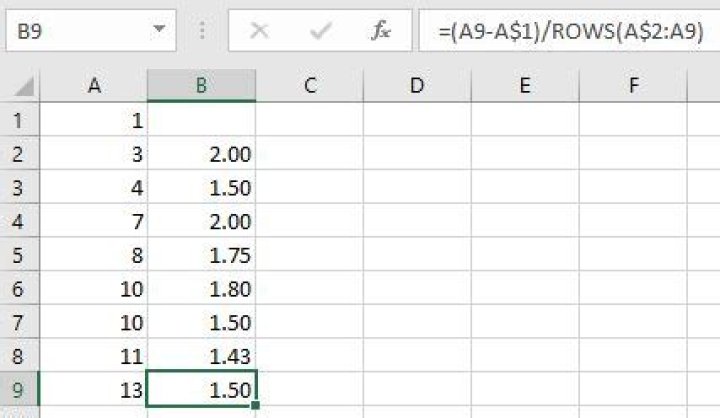
If column A includes the cumulative usage at the end of every day, you don't need to use the AVERAGE function at all. You can calculate the average by subtracting the first value from the last value and dividing by the number of days.

Enter this formula in B2 (or any empty cell in row 2)

=(A2-A$1)/ROWS(A$2:A2)

And copy it down to the other cells in the same column. B2 will now show the average daily usage after one day, C2 will show the average daily usage over the first two days, and so on.

1

I would just add a column "Delta" subtracting a1-a2 on b2, a2-a3 on b3 and so on - easy to drag & drop down ... and calculate the average of that column

1

Use an array function. For example, all the values are in column A1 to A10, the function:

={average(A1:A9-A2:A10)} 

just type "=average(A1:A9-A2:A10)"

The curly brackets show it's an array function, and you get this by holding Ctrl+Shift as you hit Enter to leave the cell.

This will give you the average difference in one cell. You could also use Sum, StdDev.S, etc.

Considering popular business practices, I would like to suggest Weighted Average method to find the forthcoming price of products in Table.

To achieve the goal you need few other information to add to the Sales Table are, Quantity Sold and Total Sale.

Below is the Sample Table along with calculated values, finds the Average Price of each product.

The mechanism behind the calculation is:

(First Day Price*First Day Qty)+(Second Day Price*Second Day Qty)+,,,/Total Qty

How it works:

• Data Range for the Sales Table is A1:E13 including Headers.

• Formula for Quantity Sold in Cell B16 is:

  =SUMIFS($D$2:$D$13,$A$2:$A$135, $A16)

• Cell C16 has Formula for Total Sale.

  =SUMIFS($E$2:$E$13,$A$2:$A$13,$A16)

• Average Price Formula in Cell D16.

  =CEILING(C16/D16,2)

N.B.

• Fill all the Formula Down.
• I've used the CEILING Function to Round up the Price, you may use ROUND or ROUNDUP also.
• Adjust cell references in the Formula as needed.

1

Your Answer

Sign up or log in

Sign up using Google Sign up using Facebook Sign up using Email and Password Submit

Post as a guest

Post Your Answer Discard

By clicking “Post Your Answer”, you agree to our terms of service, privacy policy and cookie policy