Data validation based on another cell and two column
I have a list of Food and each food has a color. Food may have multiple colors. For example, below, Banana can be Blue, Green, and Yellow, Orange can only be Green
On another cell, the user can select the Food using a dropdown. Fairly straightforward data validation. But on another, the user choose a color of that selected food. I am struggling to display a data validation for the color that is based on the available color that specific food. In other words, how to dynamically change the range of valid colors based on the selected food ?
2 Answers
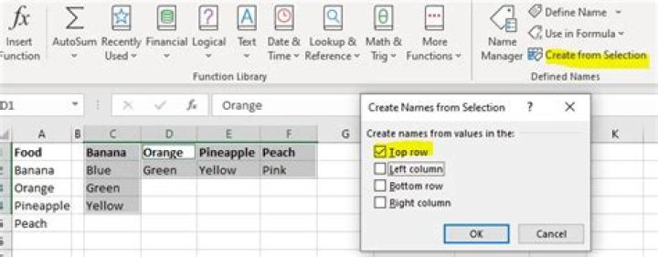
It is recommended to adjust the layout of the original data like the following picture. So we could select cells more conveniently to define names, which affects the drop down lists.
Step 1 Select cells from A1 to A5, go to Formulas > Defined Names group > Create from Selection.
Step 2 Select cells from C1 to F4, press Ctrl + G > Go To > Special > Constants > OK (It clears blanks). Do the same as Step 1 to define Names.
When going to Formulas > Name Manager in Defined Names group, we will see the Names as following.
Step 3 Select some cells under "Choose Food", go to Data > Data Tools > Data Validation, set options as following.
Step 4 Select some cells under "Choose Colors", go to Data > Data Tools > Data Validation. Enter "=INDIRECT($H2)" as Source.
Then we will get the drop list of "Banana".
You need two step solution:
Step 1:
- Get unique fruit name list.
An array (CSE) Formula in cell
F93:{=IFERROR(INDEX(F$83:F$91,MATCH(0,COUNTIF($F$92:F92,F$83:F$91),0)),"")}Create Drop down list in cell
H83, for theListtheSourceis,=$F$93:$F$97.
Step 2:
An array (CSE) formula in cell
J83, to get color's name for the fruit been selected in Drop Down.{=IFERROR(INDEX($G$83:$G$91, SMALL(IF(COUNTIF($H$83, $F$83:$F$91), ROW($F$83:$G$91)-MIN(ROW($F$83:$G$91))+1), ROW(A1)), COLUMN(A1)),"")}
N.B.
- Finish both array formula with, Ctrl+Shift+Enter, and fill down.
- Keep selecting fruits from Drop Down, to get related colors in column
J. - Adjust cell references in the formula as needed.
- For neatness, later on you may hide data in
F93:F97.