Conditional Formatting with greater than & less than parameters

I'm trying to highlight values in a column that fall between 1 and 50.

When I use the formula, =And(c3:c278>1,c3:c278=<50) none of the values that fall in between 1 and 50 are highlighted.

When I use the formula, =c3:c278<50 all values less than 50 including blank cells are highlighted.

What needs to be changed with the first formula so that it will function properly?

I assume that when a cell is blank it is still considered to have a value of 0.

1

2 Answers

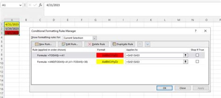
I used :

=AND(C$3:C$278>=1,C$3:C$278<=50)

and it gave :

Just dragged the formula down, did not enter it as an array formula.

4

Highlight the cells you want the conditional formatting applied to, then on the Home tab click Conditional Formatting (under styles).

The Rule Type is "Format only cells that contain", then edit the Rule Description. Choose Cell Value, Between, and type 1 and 50 in each of the respective boxes.

Lastly, choose the format you want to apply and click OK.

This should give you exactly what you want without messing around with formulas (i.e. it's foolproof). Also, blank cells aren't highlighted.

3

Your Answer

Sign up or log in

Sign up using Google Sign up using Facebook Sign up using Email and Password Submit

Post as a guest

Post Your Answer Discard

By clicking “Post Your Answer”, you agree to our terms of service, privacy policy and cookie policy